Anomalies and Counting Quark Degrees of Freedom
The article by Wally Greenberg in the spring 2015 Institute Letter mentions the anomalous axial current triangle diagram and describes its connection with counting quark degrees of freedom. This derives from a calculation I did when a long-term Member at the Institute in 1968, so I thought it would be useful to describe in detail the work done by me and by Bill Bardeen at the Institute on axial-vector or chiral anomalies. At first, this work was considered to be quantum field theory esoterica, but it has turned out to have wide and continuing implications.
But first, what is an axial-vector? A vector is a directed arrow. If you hold your right hand up to a mirror with the thumb pointing towards the mirror, you will see as the image a left hand with the thumb pointing towards you. This reversal of direction is characteristic of a vector under inversion of the coordinate axes (in this case, inversion of the axis perpendicular to the mirror). But another behavior is possible: a directed arrow that remains the same under inversion of the coordinate axes. Such a quantity is called an axial-vector or pseudovector. In the Maxwell equations for electromagnetism, electric fields behave as vectors and magnetic fields behave as axial-vectors under coordinate inversion, so this distinction has been around for many years.
Now let us fast forward to 1956, when Tsung Dao Lee (then at Columbia, later an IAS Faculty member) and Chen Ning Yang (at that time an IAS Faculty member) proposed a then-radical solution to a puzzle that had appeared in the decay of what are now called K mesons. At that time, these particles were called theta or tau mesons, depending on the decay mode, because it was assumed that inversion-symmetry or parity had to be conserved in all particle interactions. Lee and Yang studied the literature on weak interactions, and showed that there was no evidence supporting the idea of parity conservation in the weak interactions. If parity were violated (as noted at the Rochester Conference by Martin Block of Northwestern, via his roommate Richard Feynman), then a single type of meson could be decaying to final decay states with different parities. Lee and Yang proposed specific experimental tests of their suggestion, one of which was carried out by Madam Chien-Shiung Wu of Columbia and collaborators at the National Bureau of Standards, confirming in 1957 that parity is violated in weak decays. The experimental discovery of parity violation was front-page news in the New York Times. This was the year I graduated from high school, and it helped motivate my interest in particle physics. Lee and Yang received the 1957 Nobel Prize in physics for their joint work. (Much has been written about the omission of Madam Wu from Nobel recognition, which could be an essay in itself.) In the standard model of particle physics, parity violation in the weak interactions takes the form that the force carriers of the weak interactions couple to a left-handed (or left chiral) mixture of vector and axial-vector currents, in symbolic terms A-V. Under axis inversion, A does not change in sign, but V does. Under axis inversion, the coupling becomes A+V, a right handed (or right-chiral mixture) of vector and axial-vector currents.
Chiral Anomalies and π0 → γγ Decay
Let us now fast forward again to 1968, when I was a long-term Member at the Institute, having been recruited in 1966 together with Roger Dashen to restart particle theory, after IAS particle theorists Abraham Pais, Lee, and Yang left for positions elsewhere. I got into the subject of anomalies in an indirect way, through exploration during 1967–68 of the speculative idea that the muon-electron mass difference could be accounted for by giving the muon an additional electromagnetic coupling through an axial-vector current, which somehow was nonperturbatively renormalized to zero. After much fruitless study of the integral equations for the axial-vector vertex part, I decided in the spring of 1968 to first try to answer a well-defined question, which was whether the axial-vector vertex in quantum electrodynamics is renormalized by the same factor as the vector vertex, as I had been implicitly assuming. When I turned to this question, I had just started a six-week visit to the Cavendish Laboratory in Cambridge, England, after flying to London with my family in April 1968. In the laboratory, I shared an office with my former adviser Sam Treiman and was enjoying the opportunity to try a new project not requiring extensive computer analysis, unlike my thesis work on weak pion production.
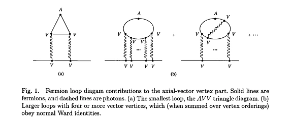
Working in the old Cavendish, I rather rapidly found an inductive multiplicative renormalizability proof, paralleling the one in the text of James Bjorken and Sidney Drell for the vector vertex. I prepared a detailed outline for a paper describing the proof, but before writing things up, I decided as a check to test whether the formal argument for the closed loop part of the Ward identity, meaning the current conservation identity, worked in the case of the smallest loop diagram. This is a triangle diagram with one axial and two vector vertices (the AVV triangle; see Fig. 1(a)), which has no analogue in the vector vertex or VVV case. I knew from a student seminar that I had attended during my graduate study at Princeton that this diagram had been explicitly calculated by Leonard Rosenberg, who was interested in the astrophysical process γV + ν → γ + ν, with γV a virtual photon emitted by a nucleus. I got Rosenberg’s paper, tested the Ward identity, and to my astonishment (and Treiman’s when I told him the result) found that it failed! I soon found that the problem was that my formal proof used a shift of integration variables inside a linearly divergent integral, which (as I again recalled from student reading) had been analyzed in an appendix to the classic text of Josef Jauch and Fritz Rohrlich, with a calculable constant remainder. For all closed loop contributions to the axial vertex in electrodynamics with larger numbers of vector vertices (the AVVVV, AVVVVVV,... loops; see Fig. 1(b)), the fermion loop integrals for fixed photon momenta are highly convergent and the shift of integration variables needed in the Ward identity is valid, so proceeding in this fermion loop-wise fashion, there were apparently no further additional or “anomalous” contributions to the axial-vector Ward identity. With this fact in the back of my mind, I was convinced from the outset that the anomalous contribution to the axial Ward identity would come just from the triangle diagram, with no renormalizations of the anomaly coefficient arising from higher order AVV diagrams with virtual photon insertions.
In early June, at the end of my six weeks in Cambridge, I returned to the United States and then went to Aspen, where I spent the summer working out a manuscript on the properties of the axial anomaly, which became the body of the final published version. Several of the things done there deserve mention, since they were important in later applications. The first was a calculation of the field theoretic form of the anomaly, giving the now well-known result
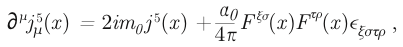
with 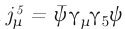
the axial-vector current (referred to above as A), F the electromagnetic field strength tensor,

the pseudoscalar current, with ε a totally antisymmetric tensor, and with m0 and α0 the (unrenormalized) fermion mass and coupling constant. In this formula, the first term on the right is the “normal” conservation result, and the second term on the right is the “anomaly,” a term I coined in my paper that has stuck. The second was a demonstration that because of the anomaly, the renormalization factor for the axial-vector vertex is not the same as that for the vector vertex (called Z2), as a result of the diagram drawn in Fig. 1(a) in which the AVV triangle is joined to an electron line with two virtual photons. Instead, the axial-vector vertex is made finite by multiplication by the renormalization constant
thus giving an answer to the question with which I started my investigation. As an application of this result, I showed that the anomaly leads, in fourth order of perturbation theory, to infinite radiative corrections to the current-current theory of νµµ and νee scattering, but that this infinity can be canceled between different fermion species by adding appropriate νµe and νeµ scattering terms to the Lagrangian. This result is a forerunner of anomaly cancelation mechanisms in modern gauge theories.
No sooner was this part of my paper completed than Sidney Coleman arrived in Aspen from Europe, and told me that John Bell and Roman Jackiw had independently discovered the anomalous behavior of the AVV triangle graph, in the context of a sigma model investigation of the Veltman–Sutherland theorem stating that π0→ γγ decay is forbidden in a calculation assuming non-anomalous behavior of the axial-vector current. Bell and Jackiw analyzed this theorem by a perturbative calculation in the sigma-model, in which the connection between normal axial-vector current conservation and pion properties is built-in from the outset, and found a non-vanishing result for the π0 → γγ amplitude, which they traced back to the fact that the regularized AVV triangle diagram cannot be defined to satisfy the requirements of both normal axial-vector and vector current conservation. This constituted the “puzzle” referred to in the title of their paper. They then proposed to modify the original sigma-model by adding further regulator fields with mass-dependent coupling constants in such a manner as to simultaneously enforce normal axial-vector and vector current conservation, thus enforcing the Sutherland–Veltman prediction of a vanishing π0 → γγγ decay amplitude.
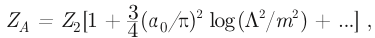
It was immediately clear to me, in the course of the conversation with Sidney Coleman, that introducing additional regulators to eliminate the anomaly would entail other problems, and was not the correct way to proceed. However, it was also clear that Bell and Jackiw had made an important observation in tying the anomaly to the Sutherland–Veltman theorem for π0 → γγγ decay, and that I could use the sigma-model version of the anomaly equation to get a nonzero prediction for the π0→ γγ amplitude, with the whole decay amplitude arising from the anomaly term! I then wrote an appendix to my paper, clearly delineated from the manuscript that I had finished before Sidney’s arrival, in which I gave a detailed rebuttal of the regulator construction, by showing that the anomaly could not be eliminated without spoiling either vector current conservation or renormalizability. (In later discussions I added unitarity to this list, to exclude the possibility of canceling the anomaly by adding a singular term to the axial current.) In this appendix, I also used an anomaly modified axial-vector current conservation equation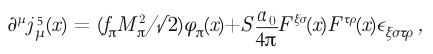
with Mπ the pion mass, φπ the pion field, and fπ the charged pion decay constant, and with S a constant determined by the neutral pion’s constituent fermion charges and axial-vector couplings, to obtain a formula for the π0 → γγγ amplitude Fπ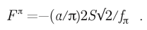
My paper was typed on my return to Princeton and was submitted to Physical Review. It was accepted along with a signed referee’s report from James Bjorken stating, “This paper opens a topic similar to the old controversies on photon mass and nature of vacuum polarization. The lesson there, as I (no doubt foolishly) predict will happen here, is that infinities in diagrams are really troublesome, and that if the cutoff that is used violates a cherished symmetry of the theory, the results do not respect the symmetry. I will also predict a long chain of papers devoted to the question the author has raised, culminating in a clever renormalizable cutoff which respects chiral symmetry and which, therefore, removes Adler’s extra term.” Thus, acceptance of the point of view that I had advocated was not immediate, but only followed over time. In 1999, Bjorken was a speaker at my sixtieth birthday conference at the Institute for Advanced Study, and he amused the audience by reading from his report, and then very graciously gave me his file copy, with an appreciative inscription, as a souvenir.
The viewpoint that the anomaly determines the π0 → γγ decay amplitude had significant physical consequences. In the appendix to my paper, I showed that the value S = 1/6 implied by the fractionally charged quark model gave a decay amplitude that was roughly a factor of 3 too small. More generally, I showed that a triplet constituent model with charges (Q, Q − 1, Q − 1) gave S = Q − 1/2 , and so with integrally charged constituents (Q = 0 or Q = 1), one gets an amplitude that agrees in absolute value, to within the expected accuracy, with experiment. This gave the first indications that neutral pion decay provides empirical evidence that can discriminate between different models for hadronic constituents. The correct interpretation of the fact that S ≃ 1/2 came only later, when what we now call the “color” degree of freedom was introduced in the seminal papers of Bill Bardeen, Harald Fritzsch, and Murray Gell-Mann and Fritzsch and Gell-Mann. These papers used my calculation of π0 → γγ decay as supporting justification for the tripling of the number of fractionally charged quark degrees of freedom, thus increasing the theoretical value of S for fractionally charged quarks from 1/6 to 1/2. The paper of Bardeen, Fritzsch, and Gell-Mann also pointed out that this tripling would show up in a measurement of R, the ratio of hadronic to muon pair production in electron positron collisions, while noting that “experiments at present are too low in energy and not accurate enough to test this prediction, but in the next year or two the situation should change,” as indeed it did.
Anomaly nonrenormalization
Before the neutral pion low-energy theorem could be used as evidence for the charge structure of quarks, one needed to be sure that there were no corrections to the anomaly and the low-energy theorem following from higher orders in perturbation theory. The fermion loop-wise argument that I used in my original treatment left me convinced that only the lowest order AVV diagram would contribute to the anomaly, but this was not a proof and was controversial. This was the motivation for a more thorough analysis of the nonrenormalization issue that I undertook with Bill Bardeen (an IAS Member at the time) in the fall and winter of 1968–69.
We approached the problem of nonrenormalization by two different methods. We first gave a general constructive argument for nonrenormalization of the anomaly to all orders, in both quantum electrodynamics and in the sigma model, and we then backed this argument up with an explicit calculation of the leading-order radiative corrections to the anomaly, showing that they canceled among the various contributing Feynman diagrams. The strategy of the general argument was to note that since the anomaly equations written above involve unrenormalized fields, masses, and coupling constants, these equations are well defined only in a cutoff field theory. Thus, for both electrodynamics and the sigma model, we constructed cutoff versions by introducing regulator fields. In the cutoff theories, the fermion loop-wise argument I used in my original anomaly paper is still valid, because regulating boson propagators does not alter the chiral symmetry properties of the theory, and thus it is straightforward to prove the validity of the anomaly equations involving unrenormalized quantities to all orders of perturbation theory.
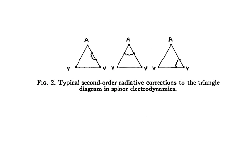
In our explicit second-order calculation, we calculated the leading-order radiative corrections to this low-energy theorem, arising from addition of a single virtual photon or virtual σ-meson to the lowest order diagram (see Fig. 2). We did this two ways, which both gave the same answer: the sum of all the radiative corrections is zero, as expected from our general nonrenormalization argument. This paper with Bardeen should have ended the controversy over whether the anomaly was renormalized, but it continued for several more years. Suffice it to say here that no objections raised have withstood careful analysis, and there is now a detailed understanding of anomaly nonrenormalization both by perturbative methods, and by nonperturbative methods proceeding from the Callan–Symanzik equations. There is also a detailed understanding of anomaly nonrenormalization in the context of supersymmetric theories, where initial apparent puzzles are now resolved.
The non-Abelian anomaly, its nonrenormalization and geometric interpretation
Since in the zero fermion mass limit the AVV triangle is identical to an AAA triangle, I knew already in unpublished notes dating from the late summer of 1968 that the AAA triangle would also have an anomaly. From fragmentary calculations begun in Aspen I suspected that higher loop diagrams might have anomalies as well, so after the nonrenormalization work was finished I suggested to Bardeen that he work out the general anomaly for larger diagrams. I showed Bill my notes, which contained a pertinent remark by Roger Dashen that including charge structure (which I had not) would allow a larger class of potentially anomalous diagrams. Within a few weeks, Bill carried out an impressive calculation of the general anomaly in both the Abelian (i.e., electromagnetic) and the non-Abelian cases. Expressed in terms of vector and axial-vector Yang-Mills field strengths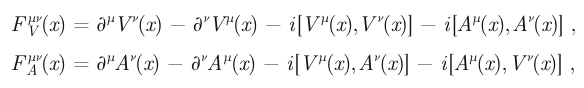
his result takes the form

= normal divergence term
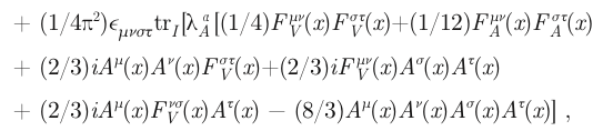
with trI denoting a trace over internal degrees of freedom, and

the internal symmetry matrix associated with the axial-vector external field. In the Abelian case, with trivial internal symmetry structure, the terms involving two or three factors of Aμ,v,... vanish by antisymmetry of ϵεμνστ, and there are only AVV and AAA triangle anomalies. When there is nontrivial internal symmetry or charge structure, there are anomalies associated with the box and pentagon diagrams as well, confirming Dashen’s intuition mentioned earlier.
There are several lines of argument leading to the conclusion that the non-Abelian chiral anomaly also has a nonrenormalization theorem, and is given exactly by the leading-order calculation. Heuristically, what is happening is that except for a few small one-fermion loop diagrams, non-Abelian theories, just like Abelian ones, are made finite by regularization of the gluon propagators. But this regularization has no effect on the chiral properties of the theory, and therefore does not change its anomaly structure, which can thus be deduced from the structure of the few small fermion loop diagrams for which naive classical manipulations break down.
The fact that non-Abelian anomalies are given by the leading-order calculation has important implications for quantum field theory. For example, the presence of anomalies spoils the renormalizability of non-Abelian gauge theories and requires the cancelation of gauged anomalies between different fermion species through imposition of the condition tr{Tα, Tβ}Tγ = 0 for all α, β, γ, with Tα the coupling matrices of gauge bosons to left-handed fermions. The fact that anomalies have a rigid structure then implies that once these anomaly cancelation conditions are imposed for the lowest-order anomalous triangle diagrams, no further conditions arise from anomalous square or pentagon diagrams, or from radiative corrections to these leading fermion loop diagrams. Anomaly cancelation is an amazing feature of the coupling structure of each family of quarks in the Standard Model, and is an important requirement in unifying extensions of the current theories.