Knots and Quantum Theory
In the twentieth century, mathematicians developed a deep theory of knots, which was revolutionized by the discovery of the Jones polynomial—a way to calculate a number for every knot—by Vaughan F. R. Jones in the early 1980s. Below, Edward Witten, Charles Simonyi Professor in the School of Natural Sciences, describes the history and development of the Jones polynomial and his interest in knot theory as a physicist.
Witten explains how the method developed by Jones and other mathematicians for comparing knots that differ by how a missing piece is filled in (as depicted by the question mark in the image above) has led to many links between the Jones polynomial and mathematical physics.
In quantum physics, a knot may be regarded as the orbit in spacetime of a charged particle. One way of calculating the Jones polynomial in quantum theory involves using the Chern-Simons function for gauge fields. But to use the Chern-Simons function, the knot must be a path in a spacetime of three dimensions (two space dimensions and one time dimension) rather than the four dimensions (three space dimensions and one dimension of time) of the real world. Beginning in the 1980s, efforts by Members in the School of Mathematics—primary among them Igor Frenkel, Louis Crane, and Michael Khovanov—have generalized the Jones polynomial to introduce a concept known as Khovanov homology, which allows the knot to become a physical object in four spacetime dimensions.
During the last decade, Sergei Gukov, Albert Schwarz, and Cumrun Vafa, former Members in the Schools of Mathematics and Natural Sciences, have developed a quantum interpretation of Khovanov homology. Witten spent the last year constructing his own approach, which involves Chern-Simons gauge theory and electric-magnetic duality and relates Khovanov homology to theories in four, five, and six dimensions. These quantum interpretations closely connect Khovanov homology to cutting-edge ideas about quantum field theory and string theory.
In everyday life, a string—such as a shoelace—is usually used to secure something or hold it in place. When we tie a knot, the purpose is to help the string do its job. All too often, we run into a complicated and tangled mess of string, but ordinarily this happens by mistake.
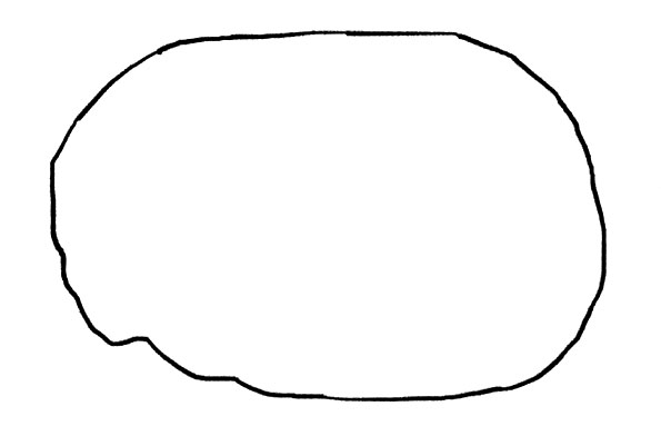
The term “knot” as it is used by mathematicians is abstracted from this experience just a little bit. A knot in the mathematical sense is a possibly tangled loop, freely floating in ordinary space. Thus, mathematicians study the tangle itself. A typical knot in the mathematical sense is shown in Figure 1. Hopefully, this picture reminds us of something we know from everyday life. It can be quite hard to make sense of a tangled piece of string—to decide whether it can be untangled and if so how. It is equally hard to decide if two tangles are equivalent.
Such questions might not sound like mathematics, if one is accustomed to thinking that mathematics is about adding, subtracting, multiplying, and dividing. But actually, in the twentieth century, mathematicians developed a rather deep theory of knots, with surprising ways to answer questions like whether a given tangle can be untangled.
But why—apart from the fact that the topic is fun—am I writing about this as a physicist? Even though knots are things that can exist in ordinary three-dimensional space, as a physicist I am only interested in them because of something surprising that was discovered in the last three decades.
Much of the theory of knots is best understood in the framework of twentieth- and twenty-first-century developments in quantum physics. In other words, what really fascinates me are not the knots per se but the connections between the knots and quantum physics. The first “knot polynomial” was actually discovered in 1923 by James W. Alexander. Alexander, a Princeton native who later was one of the original Professors at the Institute, was a pioneer of algebraic topology. But the story as I will tell it begins with the Jones polynomial, which was discovered by Vaughan F. R. Jones in 1983. The Jones polynomial was an essentially new way of studying knots. Its discovery led to a flood of new surprises that is continuing to this very day. Even though it is very modern, and near the frontier of contemporary mathematics, the Jones polynomial can be described in such a down-to-earth way that one could explain it to a high school class without compromising very much. There are not many frontier developments in modern mathematics about which one could make such a claim. For example, no one would try to explain Andrew Wiles’s proof of Fermat’s Last Theorem to high school students.
.jpg) |
| Figure 1 |
To simplify slightly (see "Some More Mathematical Details" below), what Jones discovered was a way to calculate a number for every knot. Let us call our knot K, and we will write JK for the number that Jones calculates for this knot. There is a definite rule that allows you to calculate JK for any knot. No matter how complicated K may be, one can calculate JK if one is patient enough.
If JK is not equal to 1, then the knot K can never be untangled. For example, let us go back to the knot that was sketched in Figure 1. If you were to think about how to untie that particular knot, you certainly would not succeed. But how could one prove that it is impossible? Jones gave a way to answer this sort of question: calculate JK, and if it is not equal to 1, then the knot K can never be untied. Jones’s method of computing JK was very clever, but once it was found, anyone could use it without any particular cleverness, just by following instructions.
In fact, there are an astonishing variety of ways to calculate JK. I will explain just one of the simplest. One important rule applies to the “unknot,” which is a simple untangled loop (Figure 2). If K is an unknot then JK =1.
 |
| Figure 2 |
For all other knots, we have to play a little game. To start, we pick three favorite numbers, for example 2, 3, and 10. Now we are going to do something that might seem to make life more complicated. Instead of a single knot K, we are going to consider three knots K, K', and K". If the three knots that we pick are related in a certain way, there will be an arithmetic relationship 2 JK + 3 JK' + 10 JK" = 0
This relationship—or, as mathematicians call it, this identity—is so powerful that it enables us to calculate the J’s.
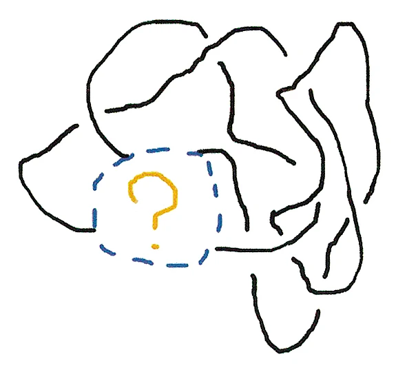
How should K, K', and K" be related in order to participate in such an identity? In Figure 3, I have drawn a partial knot. It is only a partial knot because there is a missing piece, indicated by the question mark.
.jpg) |
| Figure 3 |
There are many possible ways to complete the knot by filling in the missing piece. In Figure 4, I have sketched three of the simplest ways to do this. Choosing one of these three fillings gives us a knot that we call K, K', or K", respectively, and then, as stated previously, we declare that Jones’s numbers JK, JK', and JK" obey the relationship 2 JK + 3 JK' + 10 JK" = 0.
It turns out that this is a rather powerful relationship, which enables one to calculate JK for any K. The details of this are explained somewhat more fully in "Some More Mathematical Details" below.
.jpg) |
| Figure 4 |
The surprise here is not so much that this rule can be used to calculate JK, but that in doing this one never runs into a contradiction. One could anticipate a contradiction because actually there are many ways to use the properties that I have described to calculate JK. However, Jones and other mathematicians showed in the 1980s that there is never a contradiction—one always arrives at the same answer for JK no matter how one uses the procedure just described (or the other, related, procedures that were discovered in that period) to calculate it.
These proofs showed that the recipes for calculating JK were correct, but they left a “why” question. Unfortunately, it is not that easy to explain to someone who does not work in mathematics or physics or an allied field the difference between knowing “what” is true and knowing “why” it is true. Yet the beauty of the “why” answers is much of the reason that people do mathematics.
In this case, as people worked on the Jones polynomial, they discovered more and more remarkable formulas, with less and less clarity about what they meant.
But there was a clue. In fact, there were a lot of clues. As the subject developed, beginning with Jones’s original work, it had many ties with mathematical physics . . . bewilderingly many. If anything, too many links were found between the Jones polynomial and mathematical physics. Sometimes it is better to have one good clue than a dozen of doubtful merit!
Personally, I was most influenced during this period by the work of IAS Members Erik Verlinde, Greg Moore, and Nati Seiberg (Seiberg is now a Professor in the School of Natural Sciences) and of the Japanese mathematicians Akihiro Tsuchiya and Yukihiro Kanie, and by the suggestions of former IAS Professor Michael Atiyah.
It turned out that the explanation of the Jones polynomial has to do with quantum theory. So I need to explain a little of how quantum theory differs from pre-twentieth-century physics.
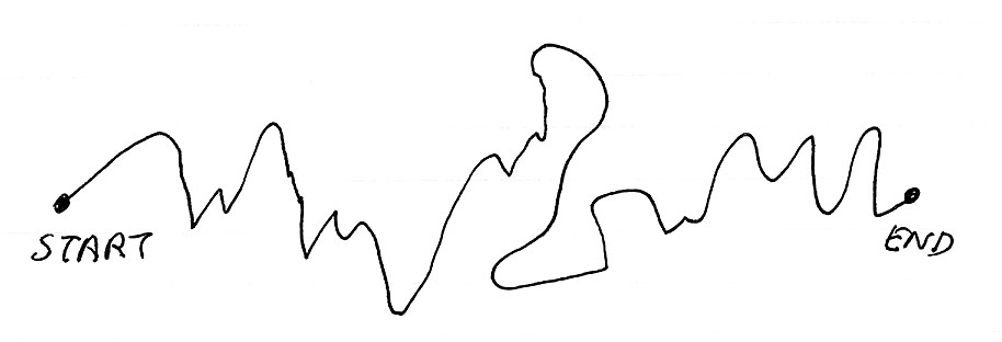
A classical particle that is traveling between one point and another gets there on a nice orbit that obeys Newton’s laws (Figure 5a). In contrast, a quantum particle can follow any path at all. A fairly typical path might be quite irregular (Figure 5b). For the quantum particle, we have to allow all possible paths, with any number of loops and zigzags.
.jpg) |
| Figure 5a |
 |
| Figure 5b |
An important point to emphasize is that we are relativistic physicists, since relativity was also invented in the twentieth century, along with quantum mechanics. So when I draw a path, it is really a path in spacetime, not a path in space.
The physical dimension of the real world we live in is therefore four—three space dimensions and one dimension of time. But to understand knot theory, at least for the moment, we are going to imagine a world of only three spacetime dimensions—two space dimensions and one time dimension.
In a world of three spacetime dimensions, the particle path might be knotted. For an example of a knotted path, see Figure 6.
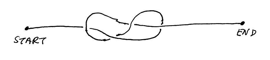 |
| Figure 6 |
A quantum physicist has to sum the effects of all possible paths by which a particle might reach its destination. How to calculate such a sum is what physicists learned in constructing quantum theory and what is now the Standard Model of particle physics.
Quantum mechanically, though any path is possible, if the particle traveled on a particular path K, then there is a “probability amplitude” for it to arrive at its destination, and this amplitude depends on K. The way that the amplitude depends on K is very important—it is the reason that there is some order even in a quantum universe. All paths are possible, but peculiar ones with a lot of zigzags are not very likely.
The quantum mechanical amplitude that the particle traveled on a path K is given by something called the Wilson operator, WK. For our purposes, we really do not need to know how it is defined. All we need to know is that it is a basic ingredient in quantum physics; for instance, physicists use it in calculating the force between quarks.
The connection between the Jones polynomial and quantum physics turns out to be simply that if we regard a knot K as the orbit in spacetime of a charged particle, then the Jones polynomial is the average value of the Wilson operator. Thus the quantum formula for the Jones polynomial is just JK = <WK>, where the symbol < > represents a process of quantum averaging.
When one carries out this program, the version of quantum theory that is relevant uses something called the Chern-Simons function for gauge fields. (Both Shiing-Shen Chern, who founded much of modern differential geometry, and James Simons, now an Institute Trustee, are former IAS Members.)
This story as I have told it so far goes back to my early years at the Institute. But there is actually a more contemporary twist to this tale. This is the reason that it seems timely to write about this topic now.
In everyday life, a knot is a physical object that exists in space, but to interpret the Jones polynomial in terms of quantum theory, we have instead had to view a knot as a path in a spacetime of only three dimensions. This is perhaps a less obvious viewpoint about what a knot means.
However, around 1990, when he was a Member at the Institute, Igor Frenkel started to develop what he hoped would be a new mathematical theory in which the knot would indeed be seen as a physical object rather than a path in spacetime. The new theory was supposed to involve a more powerful version of the Jones polynomial.
I wish I could say that I gave Frenkel some useful advice, but all I did was to tell him that it would not work because the Chern-Simons function is special to three dimensions and does not have the right sort of extension to four dimensions. It actually was a sensible objection at the time, and I am still surprised that it turned out to be wrong.
Anyway, Frenkel continued to develop this idea with, among others, his student Mikhail Khovanov and IAS Member Louis Crane. Finally, around the year 2000, Khovanov created what is now known as Khovanov homology—a refinement of the Jones polynomial in which the knot is a physical object in four spacetime dimensions rather than the path of a point particle in a spacetime of only three dimensions.
Khovanov homology is like the Jones polynomial in that once it was invented, it could be computed by an explicit set of rules, though these rules are far more sophisticated than the ones that go into the Jones polynomial. I do not think that one would try to explain the definition of Khovanov homology to high school students.
Khovanov homology has had a great deal of impact mathematically. For example, it was a major topic in a special program in the School of Math at the Institute a few years ago.
One does not need quantum physics to define Khovanov homology, though one may need quantum physics to understand what it means. Indeed, in 2004, the physicists Sergei Gukov, Albert Schwarz, and Cumrun Vafa proposed a quantum interpretation of Khovanov homology, based on the earlier work of Vafa with Hirosi Ooguri. (These physicists are all former IAS Members and/or students.) Their story used plenty of avant-garde ideas about quantum fields and strings and all that.
As beautiful and powerful as their story is, I’ve always suspected that there might be a more direct route, and I spent the last year trying to construct one. Though in a sense I succeeded, I am not sure whether to say that I found a more direct route or just a somewhat different one.1
The main difference between Khovanov homology and the Jones polynomial is that the goal of Khovanov homology is more abstract. While the Jones polynomial of a knot K is a number JK, the Khovanov homology of K is a “space of quantum states” known as HK. If you think of a knot as a physical object in three-dimensional space, then HK is the space of its possible quantum states.
Because Khovanov homology is in four spacetime dimensions rather than three, it involves ideas that are even closer to real particle physics than those that go into understanding the Jones polynomial. One important idea is symmetry between electric and magnetic fields. This is called electric-magnetic duality, and was pioneered in the 1970s by Peter Goddard (current Director of the Institute), Jean Nuyts, and David Olive (all former IAS Members). Since the mid-1990s, it has been one of the main tools in studies of quantum fields and strings, at the Institute and elsewhere. The use of electric-magnetic duality is actually crucial in circumventing the obstacle that had convinced me twenty years ago that Igor Frenkel’s idea could not work.
Another facet of string theory also turns out to be important: extra dimensions. Even though what we want is supposed to be a theory in four spacetime dimensions, it turns out that understanding it properly involves relating it to theories in five or six dimensions. The biggest surprise of all is that even though it can be defined by an explicit recipe with no reference to quantum physics—and that is how it was discovered— Khovanov homology can be understood, possibly much better, using the most modern tools of quantum field theory and string theory. Probably the full story involves physics ideas that we still do not entirely understand even today.
1 Edward Witten, “Fivebranes and Knots,” http://arxiv.org/abs/1101.3216
Some More Mathematical Details
To define the Jones polynomial (or actually a generalization of it called the HOMFLYPT polynomial) using the sort of relation described in the text, we really should introduce three variables a, b, and c and consider a general identity a JK + b JK' + c JK" = 0. By virtue of this identity (and the normalization that JK =1 for an unknot), JK turns out to be a homogeneous, rational function of the three variables.
JK is defined for a link (a disjoint union of embedded circles in three-dimensional space) and not only for a knot (a single embedded circle). In general, some or all of K, K', and K" may have more than one component. In the original Jones polynomial, the knots and links are unoriented, as shown in the illustrations that accompany this article, but in the general HOMFLYPT polynomial they are oriented.
The identity a JK + b JK' + c JK" = 0 (for every triple K, K', K" related as in Figure 4) suffices to determine the Jones polynomial of any link. This can be proved by induction in the number of crossings when the link is projected to two dimensions. For example, a knot with three crossings is sketched in Figure 7.
.jpg) |
| Figure 7 |
In the special case b=0, the relation a JK + b JK' + c JK" = 0 says that any two strands can be passed through each other while multiplying the Jones polynomial by – c/a. Of course, if strands can freely be passed through each other, we can untie any knot. For b nonzero, the relationship has an extra term, but this extra term reduces the number of crossings. So inductively, one reduces to the case that K is a link with no crossings at all—in other words, a union of s disjoint circles in the plane, for some s. A simple application of the identity a JK + b JK' + c JK" = 0 shows that in this special case, JK = (–(a+c)/b)s-1.
The proof that the identity a JK + b JK' + c JK" = 0 leads to a consistent result no matter how one applies it is less obvious, and is made by showing that the identity is consistent with certain relations among links that are known as the Reidemeister moves.
Recommended Viewing: A video of a talk on quantum theory and knots that Edward Witten gave to the Friends of the Institute for Advanced Study is available at https://www.ias.edu/video/witten-friends.