Randomness and Pseudorandomness

Computational Intractability and Pseudorandomness

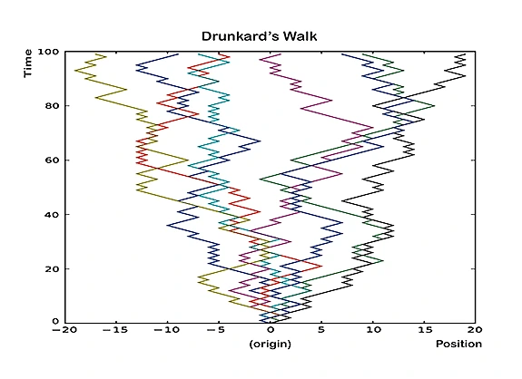
The areas of computational intractability and pseudorandomness have been among the most exciting scientific disciplines in the past decades, with remarkable achievements, challenges, and deep connections to classical mathematics. For example, the Riemann Hypothesis, one of the most important problems in mathematics, can be stated as a problem about pseudorandomness, as follows. The image above represents a “random walk” of a person or robot along a straight (horizontal) line, starting at 0. The vertical axis represents time, and each of the colored trajectories represents one instance of such a walk. In each, the robot takes 100 steps, with each step going Left or Right with probability 1/2. Note the typical distance of the walker from its origin at the end of the walk in these eight colored experiments. It is well known that for such a random (or “drunkard”) walk of n steps, the walker will almost surely be within a distance of only about √n from the origin, i.e., about ten in this case.

One can study walks under a deterministic sequence of Left/Right instructions as well, and see if they have a similar property. The Riemann Hypothesis, which probes the distribution of prime numbers in the integers, supplies such a sequence (called the Möbius sequence), roughly as follows. At each step t, walk Left if t is divisible by an odd number of distinct primes, and walk Right if it is divisible by an even number. Walking according to this sequence maintains the same distance to the origin as a typical drunkard walk if and only if the Riemann Hypothesis is true.

Research at the Institute into some of the deepest and hardest problems in the areas of computational intractability and pseudorandomness is being supported by grants from the National Science Foundation. The first, a $10 million grant, is being shared by a team of researchers at the Institute (led by Wigderson and Russell Impagliazzo, Visiting Professor), Princeton University, New York University, and Rutgers, the State University of New Jersey, which is seeking to bridge fundamental gaps in our understanding of the power and limits of efficient algorithms.

A second grant of $1.75 million is funding research directed by Jean Bourgain and Peter Sarnak, Professors in the School of Mathematics, along with Wigderson and Impagliazzo into central questions in many areas of mathematics (analysis, number theory, ergodic theory, and combinatorics) and computer science (network theory, error correction, computational complexity, and derandomization) to gain a better understanding of fundamental pseudorandomness phenomena and their interaction with structure. This has the potential to revolutionize our understanding of algorithmic processes.

Randomness and Pseudorandomness

The notion of randomness has intrigued people for millennia. Concepts like “chance,” “luck,” etc., play a major role in everyday life and in popular culture. In this article I try to be precise about the meaning and utility of randomness. In the first part I describe a variety of applications having access to perfect randomness, some of which are undoubtedly familiar to the reader. In the second part I describe pseudorandomness, the study of random-looking phenomena in non-random (or weakly random) structures, and their potential uses.

Perfect randomness and its applications
The best way to think about perfect randomness is as an (arbitrarily long) sequence of coin tosses, where each coin is fair—has a 50-50 chance of coming up heads (H) or tails (T)—and each toss is independent of all others. Thus the two sequences of outcomes of twenty coin tosses,
HHHTHTTTHTTHHTTTTTHT and
HHHHHHHHHHHHHHHHHHHH,
have exactly the same probability: 1/2²⁰.

Using a binary sequence of coin tosses as above, one can generate other random objects with a larger “alphabet,” such as tosses of a six-sided die, a roulette throw, or the perfect shuffle of a fifty-two-card deck. One of the ancient uses of randomness, which is still very prevalent, is for gambling. And indeed, when we (or the casino) compute the probabilities of winning and losing in various bets, we implicitly assume (why?) that the tosses/throws/shuffles are perfectly random. Are they? Let us look now at other applications of perfect randomness, and for each you should ask yourself (I will remind you) where the perfect randomness is coming from.

Statistics: Suppose that the entire population of the United States (over three hundred million) was voting on their preference of two options, say red and blue. If we wanted to know the exact number of people who prefer red, we would have to ask each and every one. But if we are content with an approximation, say up to a 3 percent error, then the following (far cheaper procedure) works. Pick at random a sample of two thousand people and ask only them. A mathematical theorem, called “the law of large numbers,” guarantees that with probability 99 percent, the fraction of people in the sample set who prefer red will be within 3 percent of that fraction in the entire population. Remarkably, the sample size of two thousand, which guarantees the 99 percent confidence and 3 percent error parameters, does not depend on the population size at all! The same sampling would work equally well if all the people in the world (over six billion) were voting, or even if all atoms in the universe were voting. What is crucial to the theorem is that the two thousand sample is completely random in the entire population of voters. Consider: numerous population surveys and polls as well as medical and scientific tests use such sampling—what is their source of perfect randomness?

Physics and Chemistry: Consider the following problem. You are given a region in a plane, like the one in Figure 1. A domino tiling of this region partitions the region into 2x1 rectangles—an example of such a tiling is given in Figure 2. The question is: how many different domino tilings does a given region have? Even more important is counting the number of partial tilings (allowing some holes). Despite their entertaining guise, such counting problems are at the heart of basic problems in physics and chemistry that probe the properties of matter. This problem is called the “monomer-dimer problem” and relates to the organization of di-atomic molecules on the surface of a crystal. The number of domino tilings of a given region determines the thermodynamic properties of a crystal with this shape. But even for small regions this counting problem is nontrivial, and for large ones of interest, trying all possibilities will take practically forever, even with the fastest computers. But again, if you settle for an estimate (which is usually good enough for the scientists), one can obtain such an estimate with high confidence via the so-called “Monte-Carlo method” developed by Nicholas Metropolis, Stanislaw Ulam, and John von Neumann. This is a clever probabilistic algorithm that takes a “random walk” in the land of all possible tilings, but visits only a few of them. It crucially depends on perfect random choices. In the numerous applications of this method (and many other probabilistic algorithms), where is the randomness taken from?

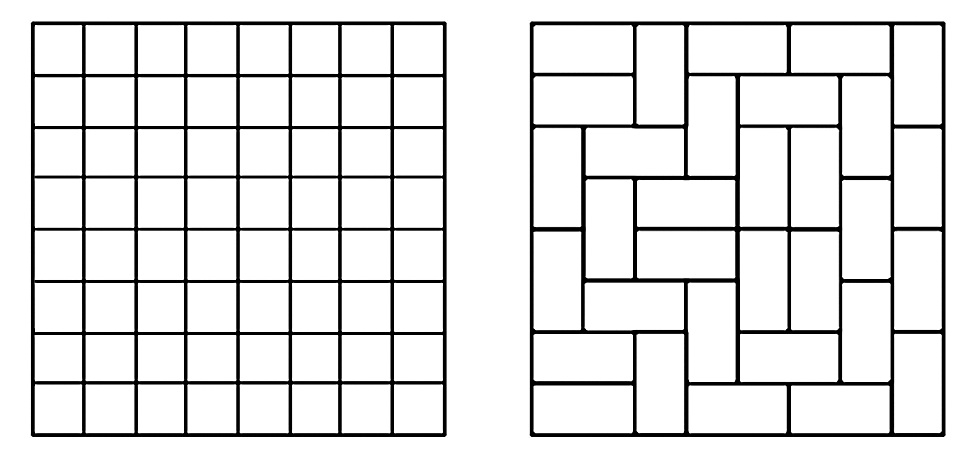
Figure 1 Figure 2

Congestion in Networks: Imagine a large network with millions of nodes and links—it can be roads, phone lines, or, best for our purpose, the Internet. When there is a large volume of traffic (cars/calls/email messages), congestion arises in nodes and links through which a lot of traffic passes. What is the best way to route traffic so as to minimize congestion? The main difficulty in this problem is that decisions as to where cars/calls/emails go are individual and uncoordinated. It is not hard to see that (in appropriate networks) if the many source-destination pairs were random, congestion would, almost surely, be quite small in every node. However, we don’t tend to choose where we go or whom we call randomly—I call my friends and you call yours, and in such cases high congestion is bound to arise. To fix this problem, Leslie Valiant proposed the following ingenious idea, which is used in practice. Whenever A wants to send an email to B, she will actually choose a random intermediate point C, send the email to C, and ask C to forward it to B (forget privacy and compliance issues—they are beside the point here). While doubling the number of email messages, Valiant proved that (in appropriate networks) the congestion drops by huge factors with very high probability. Again, perfect randomness and independence of different decisions are essential for this solution to work.

Game Theory: Sometimes the need for perfect randomness arises not for improved efficiency of some task (as in the previous examples), but for the very understanding of fundamental notions. One such notion is “rational behavior,” a cornerstone of economics and decision theory. Imagine a set of agents (e.g., people, companies, countries, etc.) engaged in a strategic interaction (e.g., traffic, price competition, cold war) in which each agent influences the outcome for everyone. Each agent has a set of optional strategies to choose from, and the choices of everyone determine the (positive or negative) value for each. All agents have this information—what set of actions then would constitute rational behavior for them all? John Nash formulated his (Nobel Prize–winning) notion of “Nash equilibrium” sixty years ago, which is widely accepted to this day. A set of strategies (one for each agent) is said to be a Nash equilibrium if no player can improve its value by switching to another strategy, given the strategies of all other agents (otherwise, it would be rational for that player to switch!). While this is a natural stability notion, the first question to ask is: which games (strategic situations as above) possess such a rational equilibrium solution? Nash proved that every game does, regardless of how many agents there are, how many strategies each has, and what value each agent obtained given everyone’s choices . . . provided that agents can toss coins! Namely, allowing mixed strategies, in which agents can (judiciously) choose at random one of their optional strategies, makes this notion universal, applicable in every game! But again, where do agents in all these situations take their coin tosses?

Cryptography: This field, which underlies all of computer security and e-commerce today, serves perhaps as the best demonstration of how essential randomness is in our lives. First and foremost, in cryptographic situations there are secrets that some know and others don’t. But what does that mean? “Secret” is another fundamental notion whose very definition requires randomness. Such a definition was given by Claude Shannon, the father of information theory, who quantified the amount of uncertainty (just how much we don’t know about it) using another fundamental notion, entropy, which necessitates that the objects at hand be random.

For example, if I pick a password completely randomly from all decimal numbers of length ten, then your chances of guessing it are precisely 1/10¹⁰. But if I choose it randomly from the set of phone numbers of my friends (also ten-digit numbers), then your uncertainty is far smaller: your probability of guessing my secret is larger, namely 1/the number of my friends (and yes, cryptography assumes that my adversaries know everything about me, except the outcomes of my coin tosses). But secrets are just the beginning: all cryptographic protocols like public-key encryption, digital signatures, electronic cash, zero-knowledge proofs, and much more, rely completely on randomness and have no secure analog in a deterministic world. You use such protocols on a daily basis when you log in, send email, shop online, etc. How does your computer toss the coins required by these protocols?

Pseudorandomness
A computational view of randomness: To answer the repeatedly asked question above, we have to carefully study our ubiquitous random object—the coin toss. Is it random? A key insight of theoretical computer science is that the answer depends on who (or which application) uses it! To demonstrate this we will conduct a few (mental) experiments. Imagine that I hold in my hand a (fair) coin, and a second after I toss it high in the air, you, as you are watching me, are supposed to guess the outcome when it lands on the floor. What is the probability that you will guess correctly? 50-50 you say? I agree! Now consider a variant of the same experiment, in which the only difference is that you can use a laptop to help you. What is the probability that you will guess correctly now? I am certain you will say 50-50 again, and I will agree again. How can the laptop help? But what if your laptop is connected to a super computer, which is in turn connected to a battery of video recorders and other sensors around the room? What are your chances of guessing correctly now? Indeed, 100 percent. It would be trivial for this machinery to calculate in one second all the required information: speed, direction, and angular momentum of the coin, the distance from my hand to the floor, air humidity, etc., and provide the outcome to you with certainty.

The coin toss remained the same in all three experiments, but the observer changed. The uncertainty about the outcome depended on the observer. Randomness is in the eye of the beholder, or more precisely, in its computational capabilities. The same holds if we toss many coins: how uncertain the outcome is to a given observer/application depends on how they process it. Thus a phenomenon (be it natural or artificial) is deemed “random enough,” or pseudorandom, if the class of observers/applications we care about cannot distinguish it from random! This viewpoint, developed by Manuel Blum, Shafi Goldwasser, Silvio Micali, and Andrew Yao in the early 1980s, marks a significant departure from older views and has led to major breakthroughs in computer science of which the field of cryptography is only one. Another is a very good understanding of the power of randomness in probabilistic algorithms, like the “Monte-Carlo method.” Is randomness actually needed by them, or are there equally efficient deterministic procedures for solving the monomer-dimer problem and its many siblings? Surprisingly, we now have strong evidence for the latter, indicating the weakness of randomness in such algorithmic settings. A theorem by Russell Impagliazzo and Wigderson shows that, assuming any natural computational problem to be intractable (something held in wide belief and related to the P=/NP conjecture), randomness has no power to enhance algorithmic efficiency! Every probabilistic algorithm can be replaced by a deterministic one with similar efficiency. Key to the proof is the construction of pseudorandom generators that produce sequences indistinguishable from random ones by these algorithms.

Random-like behavior of deterministic processes and structures: What can a clever observer do to distinguish random and non-random objects? A most natural answer would be to look for “patterns” or properties that are extremely likely in random objects, and see if the given object has them. The theorem mentioned above allows the observer to test any such property, as long as the test is efficient. But for many practical purposes, it suffices that the object has only some of these properties to be useful or interesting. Examples in both mathematics and computer science abound. Here is one: A property of a random network is that to sever it (break it into two or more large pieces), one necessarily has to sever many of its links. This property is extremely desirable in communication networks and makes them fault-tolerant. Can one construct objects with such a random-like property deterministically and efficiently?

This question has been addressed by mathematicians and computer scientists alike, with different successful constructions, e.g., by Gregory Margulis, Alexander Lubotzky, Ralph Philips, and Peter Sarnak on the math side and by Omer Reingold, Salil Vadhan, and Wigderson on the computer science side. An even more basic fault-tolerant object is an error-correcting code—a method by which a sender can encode information such that, even if subjected to some noise, a receiver can successfully remove the errors and determine the original message. Shannon defined these important objects and proved that a random code is error-correcting. But clearly for applications we need to construct one efficiently! Again, today many different deterministic constructions are known, and without them numerous applications we trust every day, from satellites to cell phones to CD and DVD players, would simply not exist!

Proving that deterministic systems and structures possess random-like properties is typically approached differently by mathematicians and computer scientists. In mathematics the processes and structures are organic to the field, arising from number theory, algebra, geometry, etc., and proving that they have random-like properties is part of understanding them. In computer science, one typically starts with the properties (which are useful in applications) and tries to efficiently construct deterministic structures that have them. These analytic and synthetic approaches often meet and enhance each other (as I will exemplify in the next section). A National Science Foundation grant to further explore and unify such connections in the study of pseudorandomness was recently awarded to Jean Bourgain, Sarnak, Impagliazzo, and Wigderson in the Institute’s School of Mathematics (see cover).

Randomness purification: Returning to the question of providing perfect randomness to all (as opposed to specific) applications, we now put no limits on the observers’ computational power. As true randomness cannot be generated deterministically, one cannot help but assume some, possibly imperfect, source of random coin tosses. Can one deterministically and efficiently convert an imperfect random source to a perfect one? How should we model imperfect randomness?

Experience with nature gives some clues. Without getting into (the interesting) philosophical discussion of whether the universe evolves deterministically or probabilistically, many phenomena we routinely observe seem at least partly unpredictable. These include the weather, stock market fluctuations, sun spots, radioactive decay, etc. Thus we can postulate, about any such phenomena, that their sequence of outcomes possesses some entropy (but where this entropy resides we have no clue). Abstractly, you can imagine an adversary who is tossing a sequence of coins, but can choose the bias of each in an arbitrary way—the probability of heads may be set to 1/2, 1/3, .99 or even 1/π, so long as it is not 0 or 1 (this would have zero entropy). Moreover, these probabilities may be correlated arbitrarily—the adversary can look at past tosses and accordingly determine the bias of the next coin. Can we efficiently use such a defective source of randomness to generate a perfect one? The (nontrivial) answer is no, as shown twenty years ago by Miklos Santha and Umesh Vazirani, who defined these sources, extending a simple model of von Neumann. But while dashing hope in one direction, they also gave hope in another, showing that if you have two (or more) such sources, which are independent of each other, then in principle one can utilize them together to deterministically generate perfect randomness. So if, for example, the weather, stock market, and sun spots do not affect each other, we can hope to combine their behavior into a perfect stream of coin tosses. What was missing was an efficient construction of such a randomness purifier (or extractor in computer science jargon).

The solution of this old problem was recently obtained using a combination of analytic and synthetic approaches by mathematicians and computer scientists. Some time ago David Zuckerman suggested the following idea: suppose A, B, and C represent the outcome of our samples of (respectively) the weather, the stock market, and sun spots (think of them as integers¹). He conjectured that the outcome of the arithmetic AxB+C would have more entropy (will be more random) than any of the inputs. If so, iterating this process (with more independent weak sources) will eventually generate a (near) perfect random number! Zuckerman proved that this concept follows from a known mathematical conjecture. While this mathematical conjecture is still open, recent progress was made on a completely different conjecture by Bourgain, Nets Katz, and Terence Tao (extending the work of Paul Erdös and Endre Szemerédi). They studied properties of random tables, and tried to find such properties in specific, arithmetic tables, namely the familiar addition and multiplication tables. Here is an intuitive description of the property they studied. Consider a small “window” in a table (see Figure 3).

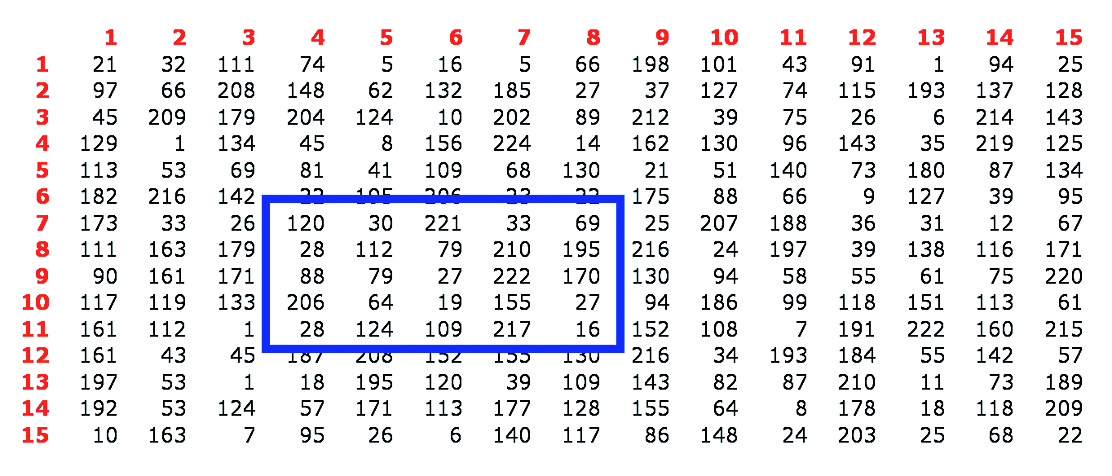
Figure 3: A random table and a typical window

Call such a window good if only a “few” of the numbers in it occur more than once. It is not hard to prove that in a random table, all small windows will be good. Now what about the addition and multiplication tables? It is very easy to see that each has bad windows!² However, Bourgain, Katz, and Tao showed that when taken together these two tables are good in the following sense (see Figure 4): for every window, it is either good in the multiplication table or in the addition table (or both)! Boaz Barak, Impagliazzo, and Wigderson gave a statistical version of this result, and used it to prove that Zuckerman’s original extractor works!

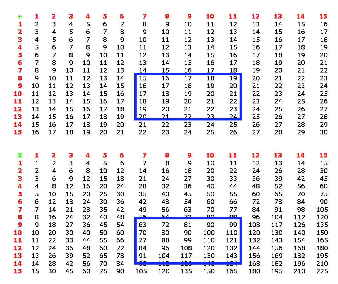
Figure 4: The addition and multiplication tables

The above story is but one example. Fundamental results from number theory and algebraic geometry, mainly on the “random-like” behavior of rational solutions to polynomial equations (by André Weil, Pierre Deligne, Enrico Bombieri, and Bourgain) were recently used in a variety of extractor constructions, purifying randomness in different settings.

Million-dollar questions on pseudorandomness: Two of the most celebrated open problems in mathematics and computer science, the Riemann Hypothesis and the P vs. NP question, can be stated as problems about pseudorandomness. These are two of the seven Clay Millennium problems, each carrying a $1 million prize for a solution (see www.claymath.org/millennium for excellent de­scrip­­tions of the problems as well as the terms for the challenge). They can be cast as problems about pseudorandomness despite the fact that randomness is not at all a part of their typical descriptions. In both cases, a concrete property of random structures is sought in specific deterministic ones.

For the P vs. NP question the connection is relatively simple to explain. The question probes the computational difficulty of natural problems. It is simple to see that random problems³ are (almost surely) hard to solve, and P vs. NP asks to prove the same for certain explicit problems, such as “the traveling salesman problem” (i.e., given a large map with distances between every pair of cities, find the shortest route going through every city exactly once).

Let’s elaborate now on the connection (explained on the cover of this issue) of the Riemann Hypothesis to pseudorandomness. Consider long sequences of the letters L, R, S, such as

S S R S L L L L L S L R R L S R R R R R S L S L S L L . . .

Such a sequence can be thought of as a set of instructions (L for Left, R for Right, S for Stay) for a person or robot walking in a straight line. Each time the next instruction moves it one unit of length Left or Right or makes it Stay. If such a sequence is chosen at random (this is sometimes called a random walk or a drunkard’s walk), then the moving object would stay relatively close to the origin with high probability: if the sequence was of n steps, almost surely its distance from the starting point would be close to √n. For the Riemann Hypothesis, the explicit sequence of instructions called the Möbius function is determined as follows for each step t. If t is divisible by any prime more than once then the instruction is Stay (e.g., t=18, which is divisible by 3²). Otherwise, if t is divisible by an even number of distinct primes, then the instruction is Right, and if by an odd number of distinct primes, the instruction is Left (e.g., for t=21=3x7 it is Right, and for t=30=2x3x5 it is Left). This explicit sequence of instructions, which is determined by the prime numbers, causes a robot to look drunk, if and only if the Riemann Hypothesis is true!

__________________

The European Association for Theoretical Computer Science and the Association for Computing Machinery Special Interest Group on Algorithms and Computation Theory recently awarded the 2009 Gödel Prize for outstanding papers in theoretical computer science to Wigderson and former Visitors Omer Reingold (1999–2003) and Salil Vadhan (2000–01). The three were selected for their development of a new type of graph product that improves the design of robust computer networks and resolves open questions on error correction and derandomization. The papers cited are “Entropy Waves, the Zig-Zag Graph Product, and New Constant Degree Expanders” by Reingold, Vadhan, and Wigderson (conceived and written at the Institute) and a subsequent paper, “Undirected Connectivity in Log-Space,” by Reingold. The prize is named for Kurt Gödel, who was a Member (1933–34, 1935, 1938, 1940–53) and Professor (1953–78) of the Institute.